
Money inflows and outflows and time
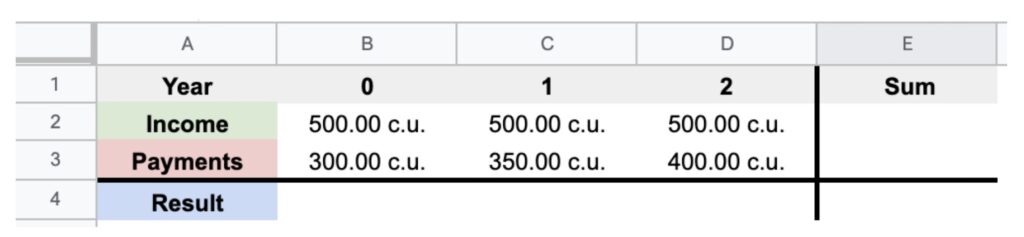
John receives an income of 500 c.u. three times: At present, in one year and in two years.
They have to face expenses of 300 c.u. at present, 350 c.u. in one year, and 400 c.u. in two years. We want to know:
- The annual result of the transaction.
- If the annual interest rate is 7%, how much are the amounts?
Firstly, we fill in the income and payments of the transaction in the spreadsheet:
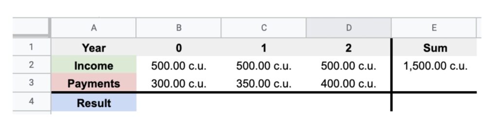
To fill in the cells, we enter the data. To calculate cell “E2” we do the following operation: “= sum (B2: D2)”.
It would look like this:
We carry out the same operation with all the empty cells, for example, to calculate the result of “D4” we would have to introduce the following formula “= D2-D3” and we get the following:
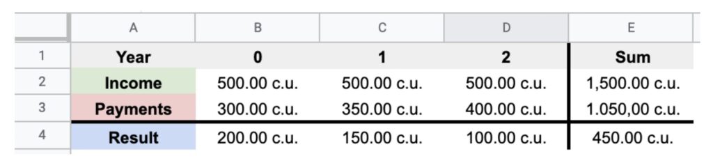
However… Are 500 c.u. in two years equal to 500 c.u. at present? No, these amounts are at different moments in time and therefore we have to take them to the same moment of time. Can we add them up? Yes, but at the same moment of time.
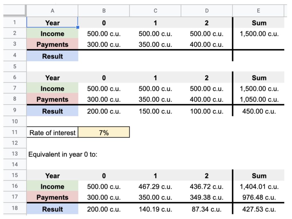
To move the amount to a moment in time we have to do:
Cell “D16” will be equal to “= D7 / ((1 + B11) ^ D6))”
Cell “D16” (income that I want to calculate in year 0) will be equal to “D7” (the corresponding amount of income) divided by (1 + “B11”/100) (cell where the interest rate is found) raised to “D6” (the year in which the time is found).
Once all the operations have been carried out, it will be as follows:
The compounding and discounting of money: Simple interest and compound interest
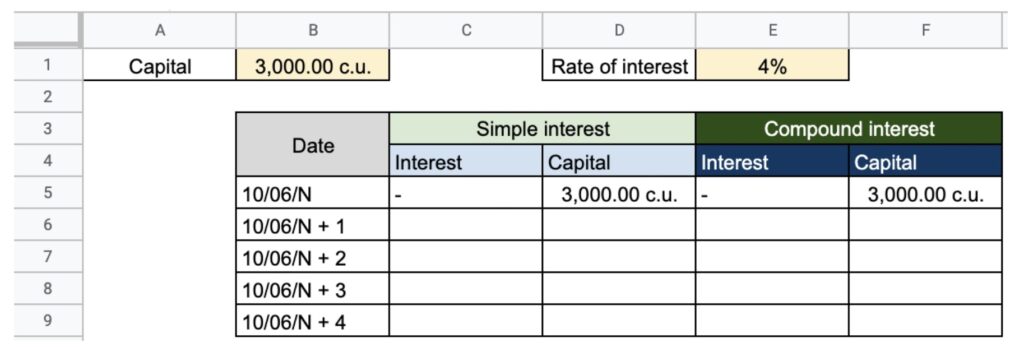
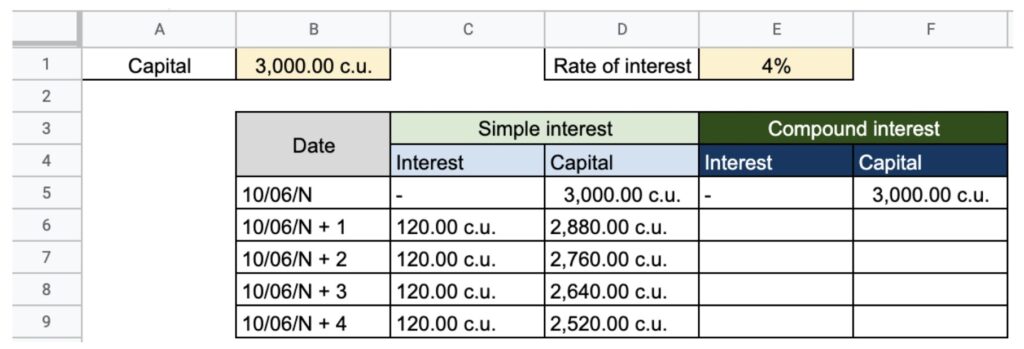
Example of capitalization: A person takes 3,000 c.u. (C) on June 10 to a financial institution that offers an annual interest of 4% (0.04 expressed in times one).
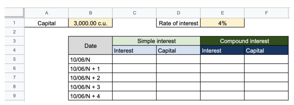
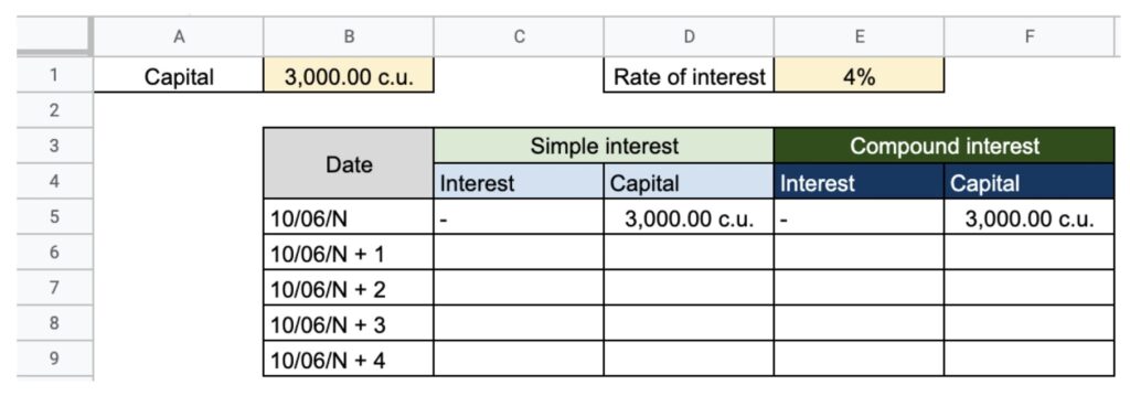
Firstly, we fill the spreadsheet with our table to position the data. We enter the initial capital and we make the calculations:
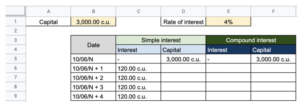
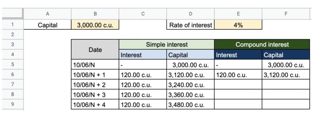
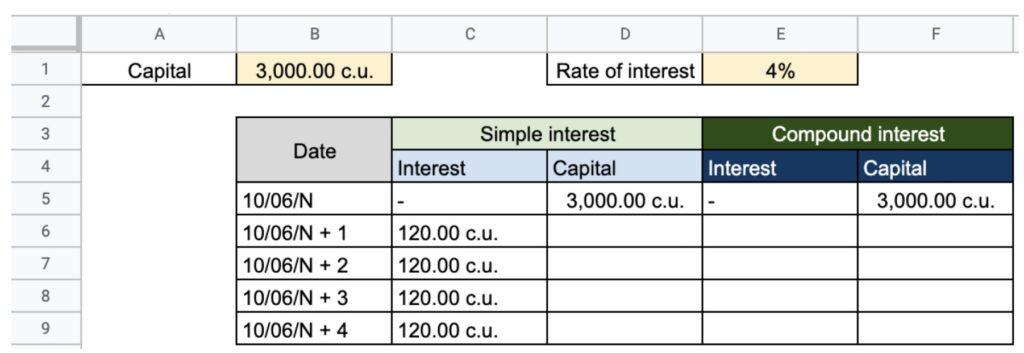
In the simple interest rate, we add the following formula in “Interest”, as they do not accumulate in the cells from “C6” to “C9” we write the following formula “= B1 * E4/100”. We multiply the capital by the interest.
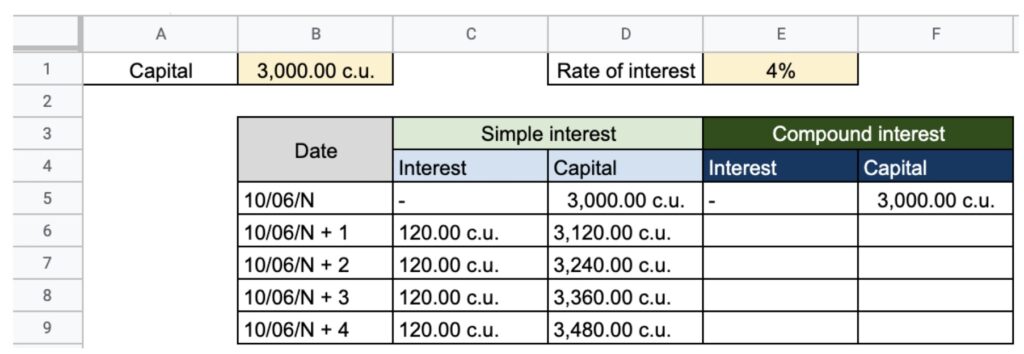
To calculate cells “D6” and later, we add the previous cell plus interest for that year. For example, to calculate cell “D6” we will have to add “D5” (capital) plus “C6” (interest): “= D5 + C6”.
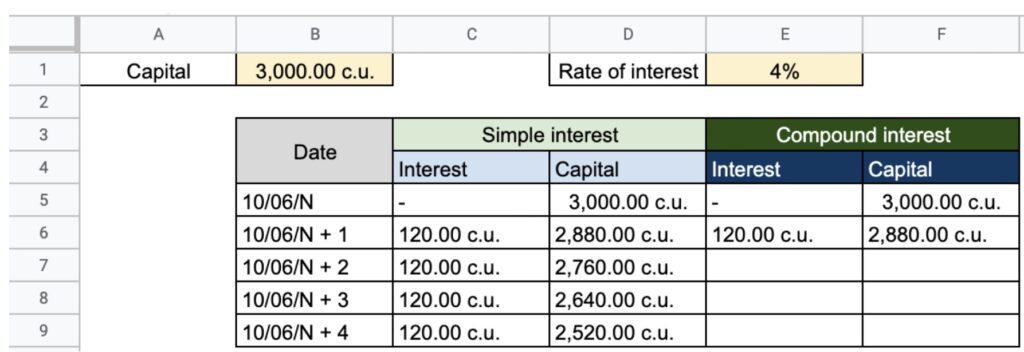
To calculate the interest on compound interest, we will have to multiply the interest rate by the capital of the previous year. In this case, to calculate the interest for the first year, we will have to apply the following formula “= F5 * 4%” and to calculate the capital for the first year “= E6 + F5”.
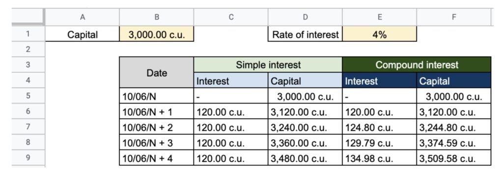
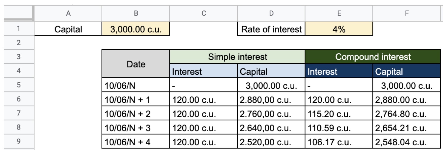
To calculate the interest for year 2 (E7), we multiply the capital at the end of time 1 by the interest “= F6 * 4%” and to calculate the capital we do the following operation “= F6 + E7”. We repeat until completing the entire table:
Discount example: A person has a bill corresponding to a capital of 3,000 c.u. to be paid on June 10 in 4 years. This person wants to cash it on June 10 of the current year and, to this end, they resort to a financial institution that offers them an annual discount of 4%.
As in the first capitalization example, we fill in the data and in the second place we calculate the interest on simple discount, as the interest to be discounted is the same in all years, we apply the following formula “= E1 * B1”:
To calculate the capital, we subtract the interest for the year in question from the initial capital; we can use the following formula for the box “D6” “= D5-C6” and so on for subsequent years:
To calculate the interest on compound discount, we have to multiply the capital of the previous year by the interest rate (4%) (“= F5 * 4%”) and we subtract them from capital (“= F5-E6”):
To calculate the interest for year 2, we multiply the capital that we get in year 1 by the interest “= F6 * 4%” and to calculate the capital of year 2, we subtract from the capital of year 1 the interest that we have calculated “= F6 – E7 ”:
Calculating the profitability of an investment
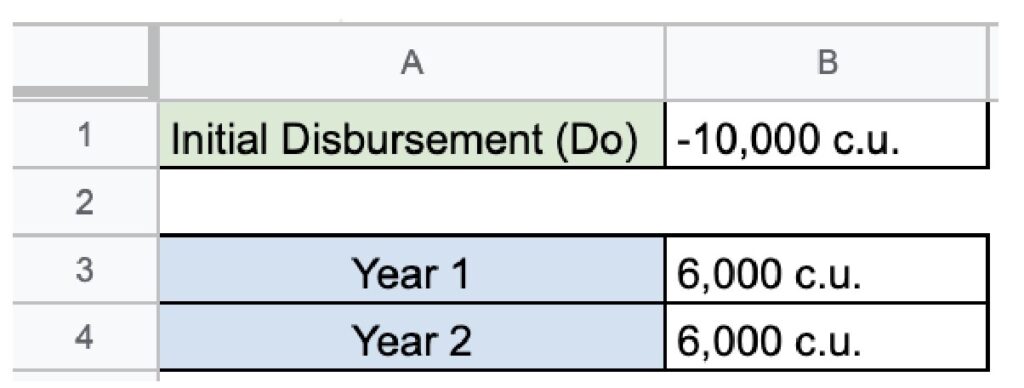
Suppose we are offered to invest in a two-year project with an initial disbursement of 10.000 c.u. and each year we will receive 6.000 c.u. Firstly, we enter the data in the spreadsheet:
Secondly, we arrange the formula:
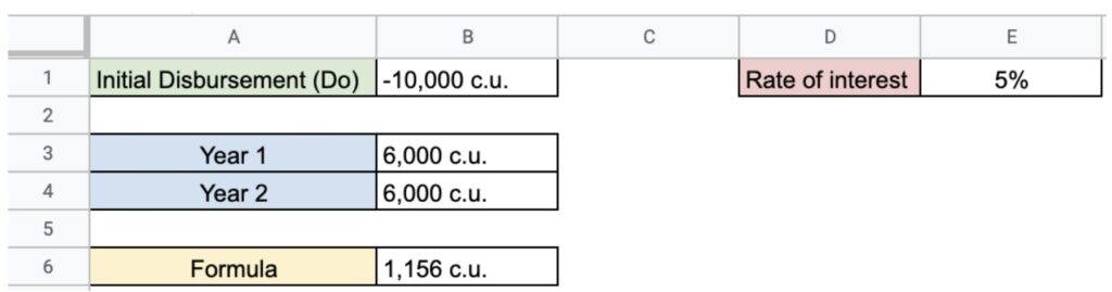
We add an interest rate, in this case 5%.
The box “B6” will be equal to the sum of B1 + C3 + C4. To calculate C3 we have to apply the following formula “= B3 / (1 + E1) ^ 1” and to calculate C4 we have to apply the following formula “= B4 / (1 + E1) ^ 2”.
Once this is done, we go to the “Data” panel, click on “What if analysis” and finally on “Search for a target…”.
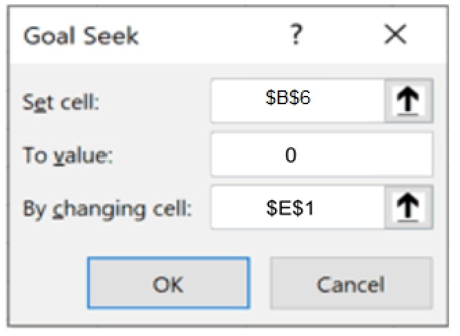
We define cell “B6” as 0 since we want it to be 0 as we have studied and to change cell “E1” which is the value we want to find.
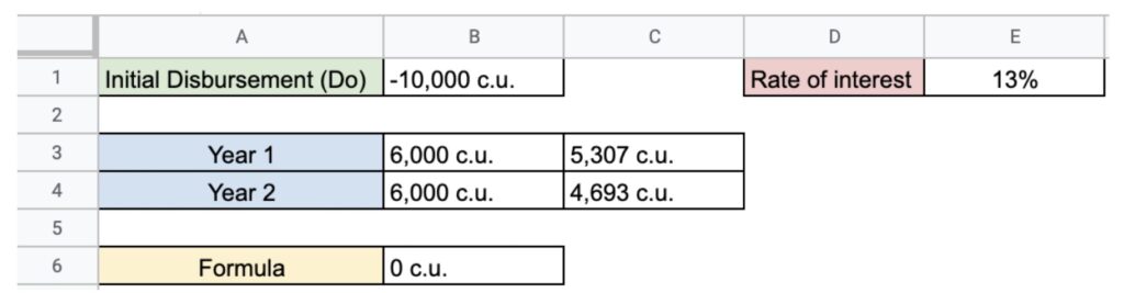
Our result is an IRR of 13,1%.
Calculating the cost of a loan
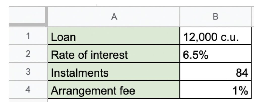
We want to take out a loan for 12,000 c.u., where:
- The interest rate is 6.5%.
- The repayment term is 7 years or 84 monthly instalments.
- The arrangement fee is 1%.
- It is paid on the last day of the month.
What is the APR of the loan?
Firstly, we enter the data:
Secondly, we calculate the instalment and, to this end, we will calculate the instalment through the “PAYMENT (PMT)” function.
“=Payment(B2/12;84;B5;0;0)”
B2 / 12: Since the interest is monthly, then it must be divided by 12.
84: Monthly instalments.
B5: The amount we have to pay is 12,120 c.u. taking into account that the fee makes part of the amount granted.
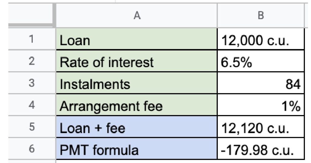
The payment function tells us we will have to pay 179.98 c.u. monthly.
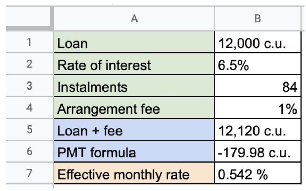
Now, we calculate the effective monthly rate and, to this end, we use the “RATE” function.
“= Rate(B3;B6;B5;0;0;0)”
B3: We add the number of instalments.
B6: We add the monthly instalment payment.
B5: We add the loan with the fee.
We get an effective monthly rate of 0.542% (6,5%/12 = 0,542%).
To calculate the APR, we have to apply the following formula:
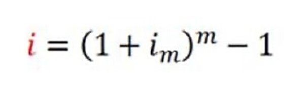
We add the following in the worksheet “= (1 + B7) (12-1)”.
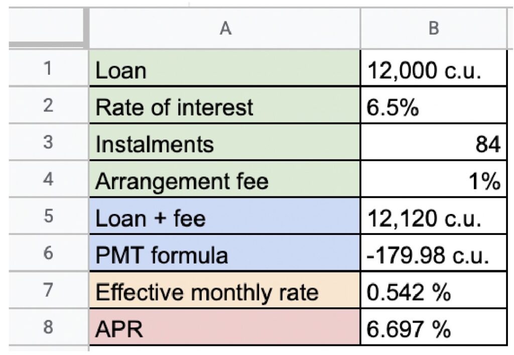
APR of the loan: 6,697%.